Matlab toolbox for estimating Phase Amplitude Coupling
Onslow AC, Bogacz R, Jones MW
Description
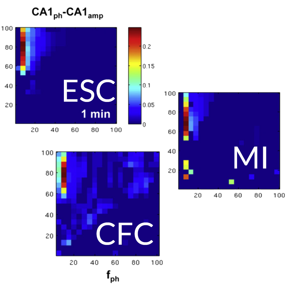
This toolbox implements three published methods for calculating Phase Amplitude Coupling (PAC):
ESC - Envelope-to-Signal Correlation (Bruns, A. and Eckhorn, R. (2004) Task-related coupling from high- to low-frequency signals among visual cortical areas in human subdural recordings. Int J Psychophysiol 51, 97-116)
MI - Modulation Index (Canolty, R. T., Edwards, E., Dalal, S. S., Soltani, M., Nagarajan, S. S., Kirsch, H. E., Berger, M. S., Barbaro, N. M. and Knight, R. T. (2006) High gamma power is phase-locked to theta oscillations in human neocortex. Science 313, 1626-8)
CFC - Cross Frequency Coupling (Osipova, D., Hermes, D. and Jensen, O. (2008) Gamma power is phase-locked to posterior alpha activity. PLoS One 3, e3990)
The main function within this tool box is find_pac_shf.m. This code compares two signals (or a single signal with itself) and creates a matrix of PAC values calulated over a range of frequency bins. This matrix is then plotted as a 'PACgram' using MATLAB's imagesc plotting function; the colour scale displays the magnitude of PAC occuring between the two signals for a given combination of frequencies.
The find_pac_shf.m function also calculates the significance of each PAC value and values which are not significant at the 5% level (default value which can be modified by the user) are set to zero and do not appear in the PACgram. If you do not want to conduct this significance analysis (this will speed up computation time) then pass the value 0 for the parameter 'num_shf' in the input to this function or alter the default value in the code.
PLEASE NOTE THAT FIND_PAC_SHF.M USES THE BONFERRONI CORRECTION FOR MULTIPLE COMPARISONS BY DEFAULT - THIS IS EASILY REMOVED BY COMMENTING OUT THE APPROPRIATE LINE OF CODE IN THIS FUNCTION WHICH IS CLEARLY LABELLED.
The function find_pac_shf_fdr.m uses a less conservative measure of correcting for multiple comparisons - by controlling the False Discovery Rate.
The function find_pac_shf_spec.m is identical to find_pac_shf.m but also plots the frequency spectrum of the signals under analysis below the PACgram.
The function find_pac_shf_tf.m calculates the time course of PAC by windowing the input signals in time and then conducting the PAC analysis (including creating shuffled data sets in order to calculate significance, unless num_shf = 0 in the input arguments). In order to plot time along the x-axis and look at the modulated higher frequency along the y-axis this function only examines the signal believed to contain the lower, modulating frequency for one frequency band of interest i.e. it looks at how that particular frequency band modulates the amplitude of all the frequency bands displayed on the y-axis (rows) of the output.
NOTE: Due to the fundamental trade-off between time and frequency resolution the length of your time window limits the lowest frequency you can accurately reconstruct: 1/length time window in seconds = lowest frequency in Hz you can reconstruct e.g if win_length = 0.5 then 2 Hz is the lowest reconstructed frequency.
NOTE: MI and ESC are better measures to use for short time windows (defined as 1s or less), CFC has frequency resolution problems but will work. It may be worth repeating any tests using the CFC measure with num_shf = 0 (i.e no significance analyis), since if the length of PAC present is the same as the length of time window used this will not be detected using the current significance analysis.
The function find_peak_freq_tf.m compares the time course of either the power spectrum of two signals or the peak frequency of two signals. It includes the option to first filter both signals for a particular frequency band of interest and then look at how the peak frequency within that band varies in time.
The function gen_simsig.m can be used to generate simulated data which contains a PAC signal occuring between two user defined frequencies. The function outputs two signals: simsig and simsigmod. The first contains the modulated amplitude envelope signal and the second contains the low frequency, modulating signal. Both signals contain a user defined level of Gaussian white noise and it is also possible for the user to specify the ratio of amplitudes between the modulated and modulating frequency component siganls.
The functions beginning sim_trials allow you to generate simulated PAC signals in trial format, with a small phase difference between each trial. The PAC signal may be set to only occur for a short period, embedded within a longer white noise signal in order to test the find_pac_shf_tf.m and find_peak_freq_tf.m functions. The frequencies involved, the amplitude of the component frequencies and the noise level can all be varied.
The funtion freq_spec.m can be used as a stand-alone function to generate a plot of the frequency spectrum of a signal. It also returns the value of the frequency with the largest power.
All other functions were written as modules to be used by the main function find_pac_shf.m. Please refer to the individual help files for each function for more details.
Assistance with this dataset
We welcome researchers wishing to reuse our data to contact the creators of datasets. If you are unfamiliar with analysing the type of data we are sharing, have questions about the acquisition methodology, need additional help understanding a file format, or are interested in collaborating with us, please get in touch via email. Our current members have email addresses on our main site. The corresponding author of an associated publication, or the first or last creator of the dataset are likely to be able to assist, but in case of uncertainty on who to contact, email Ben Micklem, Research Support Manager at the MRC BNDU.
Year Published
2019
Copyright Years
2011
Metadata
Funders
Engineering and Physical Sciences Research Council PhD studentship
Publisher
University of Oxford
Downloaded times
First Published In
2011.Prog. Biophys. Mol. Biol., 105(1-2):49-57.
Free Full Text PDF here
Group
Terms
Attribution-ShareAlike 4.0 International (CC BY-SA 4.0) This is a human-readable summary of (and not a substitute for) the licence. You are free to: Share — copy and redistribute the material in any medium or format Adapt — remix, transform, and build upon the material for any purpose, even commercially. This licence is acceptable for Free Cultural Works. The licensor cannot revoke these freedoms as long as you follow the license terms. Under the following terms: Attribution — You must give appropriate credit, provide a link to the license, and indicate if changes were made. You may do so in any reasonable manner, but not in any way that suggests the licensor endorses you or your use. ShareAlike — If you remix, transform, or build upon the material, you must distribute your contributions under the same licence as the original. No additional restrictions — You may not apply legal terms or technological measures that legally restrict others from doing anything the licence permits.