This dataset consists of a Jupyter notebook that demonstrates a tailored masked Empirical Mode Decomposition (tmEMD) workflow for local field potential (LFP) recordings using the EMD Python package; and the tailored brain region-specific masks used in Causse et al obtained using the tmEMD package.

To run it, open the notebook in Jupyter or JupyterLab and execute the cells from top to bottom. The notebook uses a synthetic pink-noise demonstration signal together with precomputed region-specific mask files used in the paper's analysis.

Data and analysis scope

The notebook is designed around a single-channel time series and a matching region-specific mask file used in the paper's analysis.

The workflow is:

1. Load a precomputed HDF5 file containing the optimized mask frequencies and iteration scores for one anatomical region used in the paper's analysis.
2. Generate a pink-noise trace as the example signal.
3. Run emd.sift.mask_sift(...) on the signal.
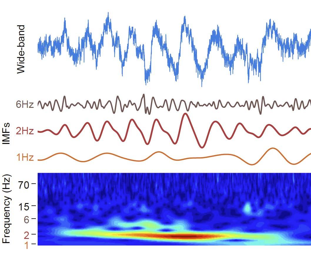
4. Compute instantaneous phase, amplitude, and frequency for the resulting IMFs.
5. Plot the trace, the IMFs, and summary spectra.

Software requirements

Install the Python packages used by the notebook:

pip install emd numpy scipy matplotlib h5py seaborn

Input files

The notebook loads a region-specific HDF5 file named:

/masks/optMaskFreqs_macro_<REGION>.h5

For the default configuration, the region is HIPPOCAMPUS, so the default file is:

/masks/optMaskFreqs_macro_HIPPOCAMPUS.h5

The file is expected to contain at least the following items:

• it_mask_freqs
• it_mix_scores
• it_consistency_scores
• info

The info object is expected to include the sample rate (sr).

Demo signal

The notebook uses pink noise as a stand-in for a real recording.

The synthetic trace is created by a call of the form:

trace = generate_pink_noise(length, freq_range=[...])

This is a controlled demo input for testing the decomposition pipeline. It is not intended to represent a biological recording.

Using a real LFP recording

To use the notebook with a real LFP file, replace the synthetic signal generation step with a loaded recording and keep the rest of the workflow unchanged.

1. Load the recording into trace

Replace the pink-noise generation line with code that loads your signal into a one-dimensional NumPy array named trace. For example:

import numpy as np

trace = np.load("my_lfp_trace.npy")

Any source format can be used as long as it is converted into a 1D array before analysis.

2. Set the sample rate

Assign the true sampling rate of the recording to sr so that the spectral and instantaneous-frequency calculations are scaled correctly:

sr = 1000  # replace with the true sampling rate

3. Select the anatomical region

The notebook uses a region label to choose the corresponding optimization file. The region names referenced in the notebook are:

• HIPPOCAMPUS
• AMYGDALA
• ENTORHINAL
• PARAHIPPOCAMPAL
• TEMPORALPOLE
• FUSIFORM
• INFERIORTEMPORAL
• MIDDLETEMPORAL
• SUPERIORTEMPORAL
• OFC
• dlPFC
• ACC

To analyze another region, change the label used in the notebook and point it to the matching HDF5 file. For example:

region = "AMYGDALA"

This would correspond to:

/masks/optMaskFreqs_macro_AMYGDALA.h5

4. Run the mask-sift analysis

Once trace, sr, and the region-specific .h5 file are set, the same decomposition and plotting steps can be applied to the real LFP recording.

Input recording format

The analysis notebook expects the LFP input to be available as a single-channel, one-dimensional numeric time series. The file format itself is flexible, provided it can be loaded into a 1D NumPy array before analysis.

Common source formats include:

• .npy
• .csv or .tsv
• .mat
• .h5
• other acquisition formats that can be converted to a 1D vector

The essential requirements are:

• one channel only
• constant sampling interval
• numeric values
• sample rate known and assigned to sr

If the recording contains multiple channels, select the channel of interest before running the notebook. If the recording is stored at a different sampling rate than the one used in the region-specific mask optimization, resample it before analysis so that the LFP trace and the mask file are matched consistently.