Overview

This website allows downloading Matlab functions generating simulated EEG data according to two theories of Event Related Potentials (ERP): the classical theory, and the phase-resetting theory. According to the classical view, peaks in ERP waveforms reflect phasic bursts of activity in one or more brain regions that are triggered by experimental events of interest. Specifically, it is assumed that an ERP-like waveform is evoked by each event, but that on any given trial this ERP "signal" is buried in ongoing EEG "noise". According the the phase-resetting theory, the experimental events reset the phase of ongoing oscillations. In particular we have implemented the method of data generation by phase-resetting proposed by Makinen et al. (2005; Neuroimage, 24:961-968).

The functions available on this website generate data in a format of the EEGLAB - a popular tool for analysis of the EEG data. This website also provides a tutorial of how to use the functions to generate the data.

The functions were used to generate data analysed in the following papers:

• Nick Yeung, Rafal Bogacz, Clay B. Holroyd and Jonathan D. Cohen. (2004) Detection of synchronized oscillations in the electroencephalogram: An evaluation of methods.Psychophysiology, 41: 822-832.
• Nick Yeung, Rafal Bogacz, Clay B. Holroyd, Sander Nieuwenhuis and Jonathan D. Cohen. (2007) Theta phase-resetting and the error-related negativity, Psychophysiology, 44: 39-49.

Installation

After downloading and decompressing the ZIP archive, the tutorial on how to use files is given below. The simulated data may be then analysed using EEGLAB.

After installing the EEGLAB please make sure to follow the instruction on how to make EEGLAB visible for Matlab (how to add path), which can be found on the EEGLAB "Download and Install" website or in the file "1ST_README.txt" in the EEGLAB.

Generating data according to the classical theory

Generating a single trial of EEG

As stated in the overview, the simulated data is generated by adding signal and noise components. These two components can be generated respectively by two functions: peak and noise. Let us first discuss generation of noise and then of the signal. Noise is generated such that its power spectrum matches the power spectrum of human EEG. In order to obtain details of parameters of function noise, one can type in Matlab (as usual):

help noise

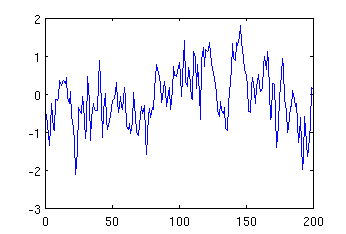
In essence this function has 3 parameters: 1st describing the length of a single trial of the signal by the number of samples, 2nd describing the number of trials, and 3rd describing sampling frequency. Hence to generate one trial of 0.8s of noise with sampling frequency 250Hz, one can type in Matlab:

mynoise = noise (200, 1, 250);

The value of the first parameters describing the number of samples was computed by multiplying the duration of the noise by the sampling frequency, i.e. 0.8 * 250 = 200. The function generates a vector containing the samples. It can be now visualised by typing:

plot (mynoise);

The resulting image may look like:

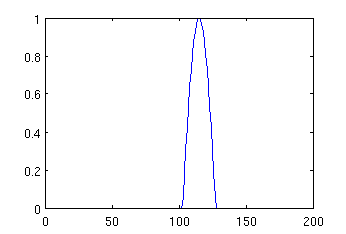
Function peak has very similar format, but it has additional parameters, including: 4th parameter describing frequency of the peak, and 5th describing position of the centre of the peak. For example, to generate a peak with frequency 5Hz and center in 115th sample, and display it, one can type:

mypeak = peak (200, 1, 250, 5, 115); plot (mypeak);

The resulting image may look like:

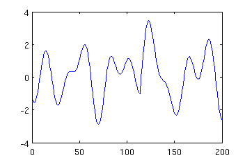
Now, once we generated both signal and noise, we can combine them. If we want to make the peak negative, we can multiply it by -1 before addition, and we can also scale the amplitudes of noise and signal by multiplying the vectors representing them before addition. For example, if we type:

mysignal = -5 * mypeak + 3 * mynoise; plot (mysignal);

the resulting image will be:

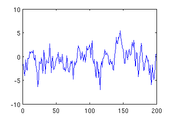
Comparing the above figure with the figure showing pure noise, one can observe that they differ around 110-120 sample due to superposition of the negative peak.

Generating complete EEG data

Function simulatedEEG generates the complete set of data (973 trials and 31 electrodes) we used in the paper "Detection of synchronized oscillations in the electroencephalogram: An evaluation of methods". See the code of this function for details, below we give the overview of main operations required to generate the complete data.

To generate multiple trials of signal, the number of trials need to be specified in the second parameter of functions peak and noise. The resulting data struture will be a vector with concatenated signals. When generating multiple trials, 6th parameter may be specified in function peak describing the temporal jitter of the peak across the trials. In order to generate data from multiple electrodes, one should generate data for each electrode separatelly and construct a matrix with a number of rows equal to the number of electrodes, in which each row correspond to the signal from one electrode. Also, one needs to remember, that the peaks have different amplitudes in different electrodes, hence they should be scaled by the co-efficients from a dipole model.

To generate sample complete set of data, type:

mydata = simulatedEEG;

Analysing simulated data

Once the data have been created (e.g. using the command above), they can be loaded to the EEGLAB. To run the EEGLAB, simply type in Matlab eeglab. To load the data, from menu "File" choose "Import data" and then "From ASCII/float file or Matlab array". In the window which opens you need to fill the following fields:

In "Data file/array" type the name of the Matlab variable with the data (e.g. "mydata", if you used mydata = simulatedEEG;).

In "Time points per epoch" type the number of samples per trial (e.g. 200, if you used simulatedEEG).

In "Data sampling rate" type the sampling rate (e.g. 250, if you used simulatedEEG).

Next to "Channel location file" click on "Browse" and find a file containing locations of electrodes (e.g. if you used simulatedEEG, the corresponding locations of electrodes are stored in file "nickloc31.locs").

and then click OK twice. Now you are ready to do analyses of the data available from menu "Plot", for example try "Channel spectra and maps".

One of the functions which can be downloaded from this website, figures, generates sample figures from the paper "Detection of synchronized oscillations in the electroencephalogram: An evaluation of methods". However, to execute this function, one first needs to add to the path the subdirectory "functions" in the "EEGLAB". Thus for example, if your EEGLAB is installed in the directory:/home/staff/rafal/linux/research/eeg/eeglab4.515, then before executing function figures, you need to type in Matlab:

addpath('/home/staff/rafal/linux/research/eeg/eeglab4.515/functions');

Generating data according to the phase-resetting theory

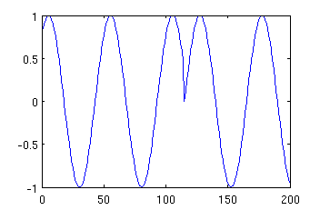
As stated in the Introduction, the phase-resetting theory assumes that the experimental events reset the phase of ongoing oscillations. Function phasereset allows to generate a sinusoid whose phase is being reset. The first three parameter of this function, are the same as for peak and noise. The next two parameters describe the minumum and maximum frequency of the oscillation - on each trial the oscillation is generated by choosing a random number from this range. The fifth parameter describes the frame in which the reset should occur. The initial phase of the oscillation is chosen randomly. Thus for example, to generate and plot the sinusoid of frequency 5 Hz being reset at 115th sample, we can type:

mysin = phasereset (200, 1, 250, 5, 5, 115); plot (mysin);

The resulting image may look like:

Makinen et al. generated their simulated data by summing 4 such sinusoids with freqencies chosen randomly from range 4-16Hz. Such data is generated by function Makinen, which has the same parameters as phasereset except the parameters describing the frequency range. Hence typing:

mysin = Makinen (200, 1, 250, 115); plot (mysin);

may result in an image like:

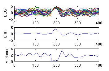
Function Makinen1a generates 30 trials of the above type, displays them, the resulting ERP and the variance in the EEG amplitude, and thus replicate Figure 1a of the paper by Makienen et al. (2005).

Have fun!